by R. Grothmann
In this notebook, we study continued fractions. A continued fraction (CF) is a way to approximate a real number with a fraction. E.g., ancient cultures used pi=22/7 as a very close approximation. How can we find such approximations?
The following is the well known CF expansion of sqrt(2) computed with the contfrac function of Euler.
>contfrac(sqrt(2),2)
[1, 2, 2]
The vector represents the fraction
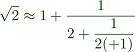
We can evaluate this, and get two approximating fractions, one with (+1) and one without.
>frac(1+1/(2+1/2)), frac(1+1/(2+1/3))
7/5
10/7
One of these approximation is the best possible rational approximation with the same or a smaller numerator.
In this case the first is the better approximation.
>1+1/(2+1/2)-sqrt(2), 1+1/(2+1/3)-sqrt(2)
-0.0142135623731
0.0143578661983
It is not difficult to get the best approximation with a fixed numerator, since
![]()
So we only have to round mx to the closest integer. The following function does this with an effort of O(m) for m<=M.
>function bestrat (x,M) ...
 nbest=round(x,0);
 mbest=1;
 err=abs(x-nbest/mbest);
 for m=2 to M;
   n=round(m*x,0);
   if abs(x-n/m)<err then
     nbest=n; mbest=m; err=abs(x-n/m);
   endif;
 end;
 return {nbest,mbest}
 endfunction
Let us test with sqrt(2) and m=7.
>{n,m}=bestrat(sqrt(2),7); n+"/"+m
7/5
The following approximation of pi has been known since ancient times.
>{n,m}=bestrat(pi,500); n+"/"+m
355/113
The algorithm to compute continued fractions works differently. It is much faster, and it can be generalized for rational functions or other fields.
The idea is to set
![]()
![]()
Then we continue recursively with r_1. floor(x) is the integer part of x, of course.
The following simple recursion does this, printing the coefficients a_i along the way.
>function docontfrac (x,n) ...
 a=floor(x),
 if n>0 then docontfrac(1/(x-a),n-1); endif;
 endfunction
>docontfrac(sqrt(2),5)
1
2
2
2
2
2
The built-in contfrac function uses a loop instead. But otherwise it works in the same way.
>contfrac(sqrt(2),5)
[1, 2, 2, 2, 2, 2]
The built-in function contfracval evaluates both approximations. It uses a loop too. The implementation is simple.
>type contfracval
function contfracval (r)
    n=cols(r);
    x1=r[n]; x2=r[n]+1;
    loop 1 to n-1
         x1=1/x1+r[n-#];
         x2=1/x2+r[n-#];
    end;
    return {x1,x2};
endfunction
It returns two real numbers. We use the frac(x) command to print them in fractional format (which in turn uses continued fractions).
>{a,b}=contfracval(contfrac(sqrt(2),5)); frac(a), frac(b),
99/70
140/99
The same for pi.
>{a,b}=contfracval(contfrac(pi,3)); frac(a), frac(b),
355/113
688/219
We can automatically choose the better one. The function fraction prints a real number as a fraction (using continued fractions internally).
>fraction contfracbest(pi,3)
355/113
The error is good enough for most earthly purposes.
>355/113-pi
2.66764189405e-007
Here is a shorter CF, which is also an ancient approximation.
>fraction contfracbest(pi,1)
22/7
>22/7-pi
0.00126448926735
The continued fraction of E has interesting coefficients. We do not prove this here, but it follows from the series of E. It can be used to show that E is transcendental.
>contfrac(E,12)
[2, 1, 2, 1, 1, 4, 1, 1, 6, 1, 1, 8, 1]
>fraction contfracbest(E,8)
1457/536
>1457/536-E
1.75363050703e-006
The CF expansion of sqrt(2) has the following explanation. The well known Newton iteration to sqrt(2) produces exactly the CF approximations, when started in 1.
>n=2; h=iterate("(x+2/x)/2",1,n), contfrac(h[-1],2*n-1)
[1,  1.5,  1.41667]
[1,  2,  2,  2]
>n=3; h=iterate("(x+2/x)/2",1,n); contfrac(h[-1],2*n-1)
[1, 2, 2, 2, 2, 2]
But the length of the approximation grows exponentially.
>n=5; h=iterate("(x+2/x)/2",1,n); contfrac(h[n],2*n-1)
[1, 2, 2, 2, 2, 2, 2, 2, 2, 2]
Let us try to compute this process in Maxima.
>function f(x) &= (x+2/x)/2
                                    2
                                x + -
                                    x
                                -----
                                  2
Maxima has an algorithm for continued fractions and its evaluation too.
>a &= f(f(f(1))), &cf(a), &ratsimp(cfdisrep(%))
                                 577
                                 ---
                                 408


                       [1, 2, 2, 2, 2, 2, 2, 2]


                                 577
                                 ---
                                 408
There is a famous approximation of the halftone interval in music.
>fracprint(contfracbest(2^(1/12),2));
18/17
It is a bit two short, when applied 12 times.
>(18/17)^12
1.98555995207
But the half tone is only 1 cent short, which is very good.
>1200*(log(18/17)-log(2^(1/12)))/log(2)
-1.04540776963
12 such half tones are 10 cent short.
>1200*(12*log(18/17)-log(2))/log(2)
-12.5448932356
This is the next best approximation.
>fracprint(contfracbest(2^(1/12),3));
107/101